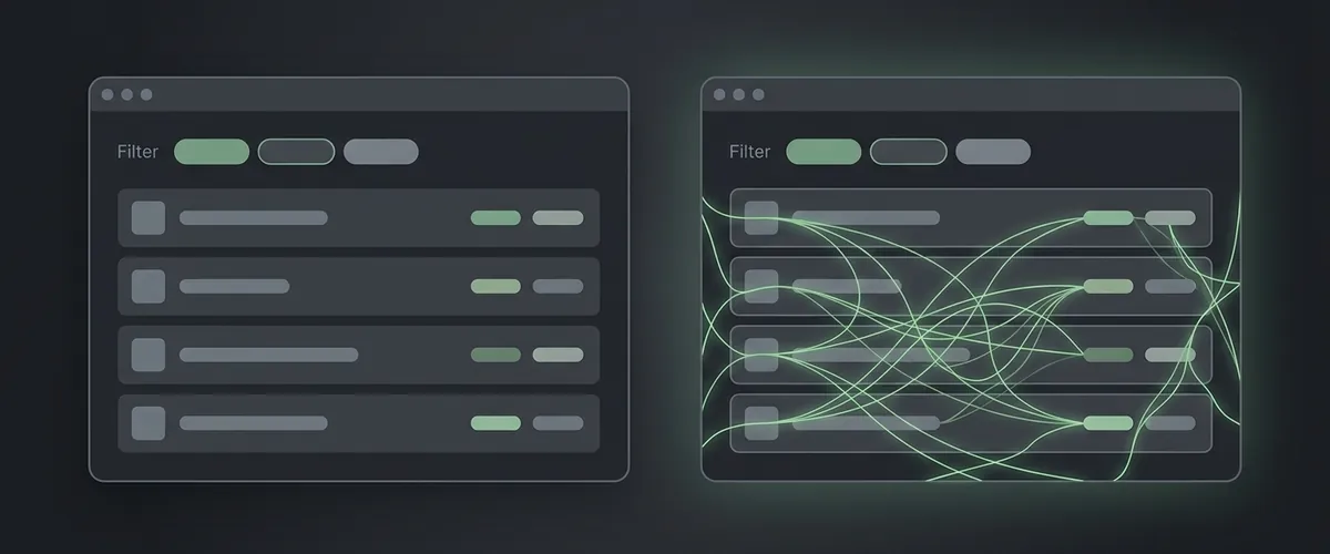
Two Models, One Token Stream
How speculative decoding pairs asymmetric models to break the memory bandwidth bottleneck.

When software engineers first learn how modern GPU hardware runs autoregressive language models, their immediate reaction is disbelief.
You provision a server equipped with an 80GB enterprise GPU capable of trillions of floating-point operations per second. You send a user prompt to a 70B parameter model, and text comes back at a pace that feels slow for hardware this expensive, on the order of tens of tokens per second.
If you profile the hardware while that stream is running, you discover that the compute cores are mostly idle. The GPU spends those cycles streaming weights from memory into the cores, not doing math.
This is the memory-bandwidth wall of generative AI. Speculative decoding finally breaks through it by running two models instead of one.
A few weeks ago I treated speculative decoding as one of three tricks that kept an aging GPU useful, and that post closed on a warning: acceptance rate is the number to check before assuming a model will feel faster. If acceptance is the whole game, what actually drives it, and what happens to the math when it collapses?
The Memory Bandwidth Trap
To understand why large models feel sluggish during generation, you have to look at the physical memory bus.
A 70B parameter model stored in 8-bit quantization weighs roughly 70GB. In autoregressive generation, generating a single token requires the GPU to read every single parameter from High Bandwidth Memory into the compute registers.
Generating Token 1: Stream 70 GB of weights from VRAM to compute cores.
Generating Token 2: Stream 70 GB of weights from VRAM to compute cores.
Generating Token 3: Stream 70 GB of weights from VRAM to compute cores.
If your GPU memory bus can transfer 2TB/s, reading 70GB of weights takes approximately 35ms. The actual matrix multiplication takes a few milliseconds. The physical speed limit of your token stream is governed by how quickly memory chips can push electrons across copper traces into the processing units.
Decades ago in CPU systems programming, hardware designers faced an identical problem: instruction fetching was slow compared to arithmetic execution. The CPU industry solved this with branch prediction and out-of-order speculative execution. The chip guessed which instructions were coming next and executed them ahead of time.
Speculative decoding brings that exact discipline to neural networks.
How Asymmetric Pairing Works
The core breakthrough was formalized by Yaniv Leviathan, Matan Kalman, and Yossi Matias at Google in their research on speculative decoding, first posted in November 2022 and published at ICML in July 2023.
Instead of forcing your 70B parameter model to generate every word sequentially, you pair it with a tiny sibling model, often in the 1B to 3B parameter range.
We call the small model the draft model and the large model the target model.
Here is what happens inside the GPU during that cycle:
First, the lightweight draft model runs 4 or 5 quick forward passes. Because the draft model is tiny, each pass reads only about 1GB of weights. Even with kernel overhead, call it 2ms per token. It speculates 5 candidate words in about 10ms.
Second, the large 70B target model takes those 5 candidate tokens and scores all 5 simultaneously in one single parallel matrix calculation. Because modern GPUs excel at batch parallel math, evaluating 5 tokens at once takes almost the exact same 35ms as evaluating one token.
Third, using a rejection-sampling step (the paper calls the scheme speculative sampling), the serving engine checks how many of the draft tokens match what the large model would have picked.
If the draft model guessed 4 of its 5 words accurately, the round yields 5 tokens (the 4 accepted plus the target’s own next token) in 45ms instead of the 175ms that 5 autoregressive passes would take.
The mathematical guarantee of speculative decoding is strict. The final token probability distribution is identical to running the large model alone, and output quality does not drop by a fraction of a percent.
The Real-World Production Trade-Offs
When speculative decoding works well, the original Google research measured 2-3x latency reductions, and production serving engines like vLLM and SGLang ship it as a standard feature. But running it in production reveals engineering trade-offs that don’t appear in research papers.
The first constraint is GPU memory overhead. You have to host both the target model and the draft model on the same physical node or GPU cluster. If your 70GB target model already pushes your 80GB GPU close to capacity, squeezing in a 3GB draft model alongside its own KV cache buffers can trigger out-of-memory errors during peak load.
The second constraint is domain alignment and acceptance rates. Speculative decoding delivers speed only when the draft model guesses correctly, and measured production traffic isn’t as accurate as the benchmarks suggest. A 29-hour trace of live production traffic published in October 2026 logged 66% of draft tokens accepted on average across 13.7M draft tokens, and controlled workloads on the same model split into a low group near 54% and a high group near 70%.
Acceptance also tracks the task. An empirical study spanning four language domains (April 2026) found that task type predicted acceptance better than speculation depth did, and only open-ended chat reliably cleared a single accepted token per step. On dense mathematical proofs, exotic internal APIs, or highly novel code, expect the low end. Engineers benchmarking speculative decoding in vLLM (April 2026) measured average acceptance sliding from 45% to 28% as they stretched the draft from 2 tokens to 4. When the large model constantly rejects the draft guesses, the extra drafting steps become pure overhead, slowing your system down rather than speeding it up.
| Workload Environment | Draft Acceptance | Speedup Outlook |
|---|---|---|
| Structured JSON / SQL | High. The draft rarely strays from the schema | Near the 2-3x the original research measured |
| Standard Web Chat | Moderate to high | Solid, around 2x |
| Dense Math / New Code | Low. Most guesses get rejected | Marginal, often a wash |
Implementing Asymmetric Serving
For engineering leaders evaluating speculative decoding across their inference infrastructure, three practical rules keep your implementations sane.
First, keep the draft model within the same architectural family. If your target model is Llama 3 70B, your draft model should ideally be Llama 3 1B or a purpose-trained speculator like EAGLE with a checkpoint trained for your target. A shared tokenizer and vocabulary is the usual starting point for high acceptance, though it is no guarantee on its own.
Second, monitor your batch size dynamics. Speculative decoding is a gift for low-batch, interactive workloads where a human is waiting on a stream. If your serving cluster handles massive batch sizes of hundreds of concurrent background jobs, the GPU naturally transitions from memory-bandwidth bound to compute-bound, which is exactly the regime where research on speculative decoding at scale finds the verification overhead erodes the speedup. At high concurrency, treat speculative decoding as a maybe, not a default.
Finally, instrument your acceptance rate as a tier-one operational metric. Treat your draft acceptance rate like a cache hit ratio. If telemetry shows acceptance dropping below 50% on a specific customer endpoint, dynamically fall back to standard autoregressive generation rather than paying speculation overhead.
We’ve spent decades learning that making systems faster rarely comes from buying faster silicon. It comes from restructuring how data moves across the bus and the wire. Speculative decoding proves that two models collaborating can outrun a single giant working alone.